When Riemann and Lebesgue aren’t enough

Why a variable mesh is all you need: Cousin’s lemma, the Kurzweil integral and its Fundamental Theorem of Calculus, generalized ODEs, and why measure differential equations are generalized ODEs.

Author

Affiliation

Lucas Ozaki Mizuguti

IBILCE-UNESP

Integration theories can be sorted by the way they treat cancellation. The Lebesgue integral is absolute: a measurable function \(f\) is integrable if and only if \(|f|\) is. This is the integral analogue of absolute convergence of series, and it has the same blind spot. A function whose integral exists only because its positive and negative parts cancel, such as a derivative that oscillates faster and faster, is out of reach, just as a conditionally convergent series is not absolutely convergent. An integral is called non-absolute when \(f\) may be integrable while \(|f|\) is not. The first non-absolute integrals, due to Denjoy (1912) and Perron (1914), integrate every derivative, but they are defined by transfinite induction and by major and minor functions, far from the Riemann sums of elementary calculus.

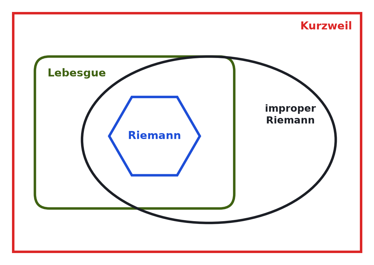
In 1957, while looking for optimal conditions for the continuous dependence of solutions of ordinary differential equations on parameters, Kurzweil (Kurzweil 1957) found a definition of Riemann type. He kept the Riemann sums and changed only the way the fineness of a tagged division is measured: instead of a single number, the mesh, he used a positive function \(\delta\), called a gauge, so that the allowed size of each piece depends on where it is. Henstock introduced the same idea independently in 1961 (Henstock 1961). For real functions on \([a,b]\), the resulting Kurzweil integral coincides with the Perron integral; it contains the Lebesgue integral and the improper Riemann integral, and \(f\) is Lebesgue integrable if and only if both \(f\) and \(|f|\) are Kurzweil integrable (Gordon 1994).

import matplotlib.pyplot as plt
from matplotlib.patches import Ellipse, FancyBboxPatch, Rectangle, RegularPolygon

RED, GREEN, BLACK, BLUE = "#dc2626", "#3f6212", "#1c1f26", "#1d4ed8"

fig, ax = plt.subplots(figsize=(7, 4.6))
ax.set_xlim(0, 10)
ax.set_ylim(0, 7)
ax.set_aspect("equal")
ax.axis("off")

# the four classes of integrable functions
ax.add_patch(Rectangle((0.2, 0.2), 9.6, 6.6, fill=False, ec=RED, lw=3))                    # Kurzweil
ax.add_patch(FancyBboxPatch((0.8, 1.4), 5.5, 4.2, boxstyle="round,pad=0,rounding_size=0.4",
                            fill=False, ec=GREEN, lw=3))                                    # Lebesgue
ax.add_patch(Ellipse((5.6, 3.3), 7.0, 4.6, fill=False, ec=BLACK, lw=3))                     # improper Riemann
ax.add_patch(RegularPolygon((4.1, 3.4), numVertices=6, radius=1.25, orientation=0.5236,
                            fill=False, ec=BLUE, lw=3))                                     # Riemann

ax.text(9.55, 6.35, "Kurzweil", color=RED, fontsize=13, fontweight="bold", ha="right")
ax.text(1.15, 5.05, "Lebesgue", color=GREEN, fontsize=13, fontweight="bold")
ax.text(7.85, 3.75, "improper\nRiemann", color=BLACK, fontsize=12, fontweight="bold", ha="center")
ax.text(4.1, 3.4, "Riemann", color=BLUE, fontsize=13, fontweight="bold", ha="center", va="center")

fig.tight_layout()
plt.show()

Figure 1: Integrable functions on \([0,1]\). Every Riemann integrable function is Lebesgue integrable and improper Riemann integrable, and both of these classes are contained in the Kurzweil integrable functions (for the improper integral, by the Hake-type theorem (Bonotto et al. 2021, Theorem 2.9)).

Kurzweil’s integral was born together with an application. Its sums \(\sum_i\bigl[U(\tau_i,s_i)-U(\tau_i,s_{i-1})\bigr]\) integrate functions of two variables, and with them Kurzweil defined generalized ordinary differential equations. These are integral equations whose solutions may be discontinuous, and they contain classical ODEs, measure differential equations, impulsive equations and dynamic equations on time scales as particular cases (Schwabik 1992; Bonotto et al. 2021).

The objective of this note is to give a brief but precise introduction to the theory of the Kurzweil integral and of generalized ODEs, and to their relation with measure differential equations. We introduce gauges and prove Cousin’s lemma (Lemma 1); define the Kurzweil integral (Definition 3) and prove its basic properties (Theorem 1) and the Fundamental Theorem of Calculus (Theorem 2); define generalized ODEs; and show that measure differential equations are generalized ODEs (Theorem 4).

Gauges and \(\delta\)-fine division

In what follows, we define the concepts of tagged division and a gauge with respect to a compact interval of the real line.

Definition 1 (Tagged division) A tagged division of a compact interval \([a,b] \subset \mathbb{R}\) is a finite collection of point-interval pairs \[ D = \left\{(\tau_{i},[s_{i-1},s_{i}]) \colon i = 1,2,\dots, |D|\right\}, \] where \(a = s_{0} \le s_{1} \le \dots \le s_{|D|} = b\) constitutes a partition of \([a,b]\), \(|D|\) denotes the number of subintervals \([s_{i-1}, s_{i}]\), and \(\tau_{i} \in [s_{i-1},s_{i}]\) is a designated tag for the subinterval \([s_{i-1}, s_{i}]\) for each \(i \in \{1,2,\dots, |D|\}\).

Definition 2 A strictly positive function \(\delta \colon [a,b] \to (0, \infty)\) is called a gauge on \([a, b]\). Given a gauge \(\delta\) on \([a, b]\), a tagged division \(D = \left\{(\tau_{i},[s_{i-1},s_{i}]) \colon i = 1,2,\dots,|D|\right\}\) of \([a,b]\) is said to be \(\delta\)-fine if \[ [s_{i-1},s_{i}] \subset (\tau_{i} - \delta(\tau_{i}), \tau_{i} + \delta(\tau_{i})) \quad \text{for every } i \in \{1,2,\dots, |D|\}. \]

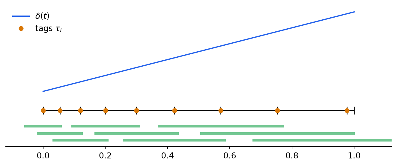
Where \(\delta\) is small the division is forced to be fine; where \(\delta\) is large it can be coarse. Figure 2 shows a \(\delta\)-fine division for \(\delta(t)=0.06+0.25\,t\) on \([0,1]\), built greedily from the left.¹

¹ The animated version builds the same division one pair at a time.

import matplotlib.pyplot as plt
import numpy as np

delta = lambda t: 0.06 + 0.25 * t

points, tags, s = [0.0], [], 0.0
while s < 1:
    tags.append(s)
    s = min(1.0, s + 0.9 * delta(s))
    points.append(s)

fig, ax = plt.subplots(figsize=(7, 3))
t = np.linspace(0, 1, 200)
ax.plot(t, delta(t), color="#2563eb", label=r"$\delta(t)$")
ax.hlines(0, 0, 1, color="black", lw=1)
ax.vlines(points, -0.012, 0.012, color="black", lw=1)
ax.plot(tags, np.zeros_like(tags), "o", color="#d97706", ms=5, label=r"tags $\tau_i$")
for i, tau in enumerate(tags):
    y = -0.05 - 0.022 * (i % 3)
    ax.hlines(y, tau - delta(tau), tau + delta(tau), color="#16a34a", lw=3, alpha=0.6)
ax.set_xlim(-0.12, 1.12)
ax.set_yticks([])
ax.spines[["left", "right", "top"]].set_visible(False)
ax.legend(frameon=False, loc="upper left")
fig.tight_layout()
plt.show()

Figure 2: A \(\delta\)-fine tagged division of \([0,1]\). Each bar below the axis is the interval \((\tau_i-\delta(\tau_i),\tau_i+\delta(\tau_i))\), which must contain the \(i\)-th subinterval.

The choice of the tags matters: the same partition can give a \(\delta\)-fine tagged division with some tags and not with others.

Example 1 (Not every choice of tags is \(\delta\)-fine) Consider the partition \[ P=\left\{\left[0,\tfrac{1}{3}\right],\left[\tfrac{1}{3},\tfrac{1}{2}\right],\left[\tfrac{1}{2},1\right]\right\} \] of \([0,1]\) and the gauge \(\delta\colon[0,1]\to(0,1]\) given by \[ \delta(t)=\begin{cases} t, & 0<t\le 1,\\[2pt] \tfrac{1}{2}, & t=0. \end{cases} \] The tagged division \[ D=\left\{\left(\tfrac{1}{10},\left[0,\tfrac{1}{3}\right]\right),\ \left(\tfrac{1}{2},\left[\tfrac{1}{3},\tfrac{1}{2}\right]\right),\ \left(1,\left[\tfrac{1}{2},1\right]\right)\right\} \] is not \(\delta\)-fine, because \[ \left[0,\tfrac{1}{3}\right]\not\subset\left(\tfrac{1}{10}-\delta\left(\tfrac{1}{10}\right),\ \tfrac{1}{10}+\delta\left(\tfrac{1}{10}\right)\right)=\left(0,\tfrac{1}{5}\right). \]

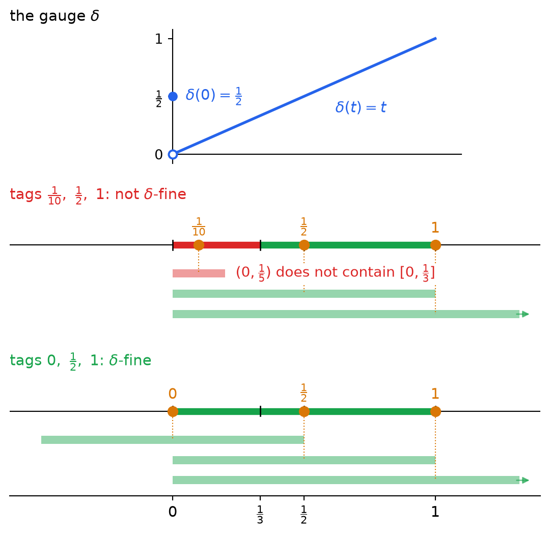
The other two pairs of \(D\) are fine: \(\left(\tfrac{1}{2}-\delta(\tfrac{1}{2}),\tfrac{1}{2}+\delta(\tfrac{1}{2})\right)=(0,1)\) contains \(\left[\tfrac{1}{3},\tfrac{1}{2}\right]\), and \(\left(1-\delta(1),1+\delta(1)\right)=(0,2)\) contains \(\left[\tfrac{1}{2},1\right]\). Only the first tag is a problem. Moving it to \(0\) fixes it, since \(\left(-\tfrac{1}{2},\tfrac{1}{2}\right)\supset\left[0,\tfrac{1}{3}\right]\), so the tags \(0,\tfrac{1}{2},1\) give a \(\delta\)-fine tagged division (Figure 3). In fact \(0\) is the only tag that works for a subinterval containing \(0\): for \(\tau>0\) we have \((\tau-\delta(\tau),\tau+\delta(\tau))=(0,2\tau)\), which never contains \(0\). A gauge can force the position of a tag in this way.

import matplotlib.pyplot as plt
import numpy as np


def delta(t):
    """The gauge of the example: delta(t) = t for 0 < t <= 1, and delta(0) = 1/2."""
    return 0.5 if t == 0 else t


s = [0, 1 / 3, 1 / 2, 1]          # the partition P of [0, 1]
tags_D = [1 / 10, 1 / 2, 1]       # the tags of D (as in the example)
tags_E = [0, 1 / 2, 1]            # the same partition, first tag moved to 0

GREEN, RED, BLUE, ORANGE = "#16a34a", "#dc2626", "#2563eb", "#d97706"
XMIN, XMAX = -0.62, 1.32
TICKS = {0: "0", 1 / 3: r"$\frac{1}{3}$", 1 / 2: r"$\frac{1}{2}$", 1: "1"}
TAG_TEXT = {0: "0", 1 / 10: r"$\frac{1}{10}$", 1 / 2: r"$\frac{1}{2}$", 1: "1"}

fig, axes = plt.subplots(3, 1, figsize=(7, 6.2), sharex=True,
                         gridspec_kw={"height_ratios": [1.1, 1, 1], "hspace": 0.35})

# (a) the gauge: a jump at t = 0
ax = axes[0]
t = np.linspace(0, 1, 200)
ax.plot(t, t, color=BLUE, lw=2)
ax.plot([0], [0], "o", ms=6, mfc="white", mec=BLUE, mew=1.5, zorder=3)   # delta(0) is not 0 ...
ax.plot([0], [0.5], "o", ms=6, color=BLUE, zorder=3)                     # ... it is 1/2
ax.text(0.05, 0.5, r"$\delta(0)=\frac{1}{2}$", color=BLUE, fontsize=11, va="center")   # a single point
ax.text(0.62, 0.36, r"$\delta(t)=t$", color=BLUE, fontsize=11)
ax.plot([0, 1.1], [0, 0], color="black", lw=0.8)     # the gauge is only defined on [0, 1]
ax.set_ylim(-0.08, 1.08)
ax.set_yticks([0, 0.5, 1], ["0", r"$\frac{1}{2}$", "1"])
ax.set_title("the gauge $\\delta$", loc="left", fontsize=11)


def draw(ax, tags, title):
    """The partition on a line; under it, the interval (tau_i - delta(tau_i), tau_i + delta(tau_i)) of each tag."""
    ax.axhline(0, color="black", lw=0.8)
    fine = True
    for i, tau in enumerate(tags):
        u, v, d = s[i], s[i + 1], delta(tau)
        ok = tau - d < u and v < tau + d          # [u, v] inside the open interval (tau - d, tau + d)
        fine &= ok
        col = GREEN if ok else RED
        ax.plot([u, v], [0, 0], color=col, lw=5, solid_capstyle="butt")
        y = -0.42 - 0.3 * i
        lo, hi = max(tau - d, XMIN), min(tau + d, XMAX)
        ax.plot([lo, hi], [y, y], color=col, lw=6, alpha=0.45, solid_capstyle="butt")
        if tau + d > XMAX:                          # the interval goes on beyond the picture
            ax.annotate("", (XMAX + 0.05, y), (XMAX - 0.02, y),
                        arrowprops=dict(arrowstyle="-|>", color=col, alpha=0.6))
        ax.plot([tau, tau], [0, y], color=ORANGE, lw=0.8, ls=":")
        ax.plot([tau], [0], "o", color=ORANGE, ms=7, zorder=3)
        ax.text(tau, 0.13, TAG_TEXT[tau], color=ORANGE, ha="center", va="bottom", fontsize=11)
        if not ok:
            ax.text(tau + d + 0.04, y, r"$(0,\frac{1}{5})$ does not contain $[0,\frac{1}{3}]$", color=RED,
                    va="center", fontsize=10.5, bbox=dict(facecolor="white", edgecolor="none", pad=1))
    for x in s:
        ax.plot([x, x], [-0.07, 0.07], color="black", lw=1)
    ax.set_ylim(-1.25, 0.55)
    ax.set_yticks([])
    verdict = r"$\delta$-fine" if fine else r"not $\delta$-fine"
    ax.set_title(f"{title}: {verdict}", loc="left", fontsize=11, color=GREEN if fine else RED)


draw(axes[1], tags_D, r"tags $\frac{1}{10},\ \frac{1}{2},\ 1$")
draw(axes[2], tags_E, r"tags $0,\ \frac{1}{2},\ 1$")

for ax in axes:
    ax.spines[["left", "right", "top"]].set_visible(False)
axes[0].spines["left"].set_visible(True)
axes[0].spines["left"].set_position(("data", 0))     # vertical axis at t = 0
for ax in axes[:2]:
    ax.spines["bottom"].set_visible(False)
    ax.tick_params(axis="x", bottom=False)
axes[2].set_xticks(list(TICKS), list(TICKS.values()))
axes[2].tick_params(axis="x", labelsize=11)
axes[2].set_xlim(XMIN, XMAX + 0.08)
plt.show()

Figure 3: Example 1. Top: the gauge \(\delta\) on \([0,1]\), equal to \(\frac{1}{2}\) at the single point \(t=0\) (filled dot) and to \(t\) for \(0<t\le1\). Middle and bottom: the partition \(P\) with two choices of tags (orange). Each bar is the interval \((\tau_i-\delta(\tau_i),\tau_i+\delta(\tau_i))\), which must contain the \(i\)-th subinterval; an arrow means the interval continues beyond the picture.

The definition would be useless if fine divisions could fail to exist. They cannot:

Lemma 1 (Cousin’s lemma) For every gauge \(\delta\) on \([a,b]\) there exists a \(\delta\)-fine tagged division of \([a,b]\).

Proof. Suppose not. If both halves of \([a,b]\) had \(\delta\)-fine tagged divisions, their union would be one for \([a,b]\); hence some half \(I_1\) has none. Repeating the argument gives nested closed intervals \(I_1\supset I_2\supset\cdots\) with \(|I_n|=(b-a)/2^n\), none of which admits a \(\delta\)-fine tagged division. Let \(c\) be the point in \(\bigcap_n I_n\) and choose \(n\) with \((b-a)/2^n<\delta(c)\). Since \(c\in I_n\), we get \(I_n\subset(c-\delta(c),c+\delta(c))\), so \(\{(c,I_n)\}\) is a \(\delta\)-fine tagged division of \(I_n\), a contradiction.

The Kurzweil integral

Let \(X\) be a Banach space.

Definition 3 (Kurzweil integral) A function \(U\colon[a,b]\times[a,b]\to X\) is called Kurzweil integrable over \([a,b]\), if there exists an element \(\mathcal{I}\in X\) such that for each \(\epsilon>0\), there is a gauge \(\delta\) on \([a,b]\) such that \[ \left\|\sum_{i=1}^{|D|}\left[U(\tau_{i},s_{i})-U(\tau_{i},s_{i-1})\right]-\mathcal{I}\right\| < \varepsilon, \] for every \(\delta\)-fine tagged division \(D=\{(\tau_{i},[s_{i-1},s_{i}])\colon i=1,2,\dots,|D|\}\), of \([a,b]\). In this case, \(\mathcal{I}\) is called the Kurzweil integral of \(U\) over \([a,b]\) which will be denoted by \(\int_{a}^{b}DU(\tau,t)\).

When the Kurzweil integral \(\int_{a}^{b}DU(\tau,t)\) exists, we define \[ \int_{a}^{b}DU(\tau,t) = -\int_{b}^{a}DU(\tau,t) \quad \text{and} \quad \int_{a}^{a}DU(\tau,t) = 0. \]

Remark 1 (Particular case). In the case where \[ U(\tau, t) = f(\tau)\, g(t), \qquad \tau, t \in [a,b], \] with \(f \colon [a,b] \to X\) and \(g \colon [a,b] \to \mathbb{R}\), in Definition 3, we obtain \[ \sum_{i=1}^{|D|} \bigl[ U(\tau_i, s_i) - U(\tau_i, s_{i-1}) \bigr] = \sum_{i=1}^{|D|} f(\tau_i)\, \bigl( g(s_i) - g(s_{i-1}) \bigr), \] where \(D = \{ (\tau_i, [s_{i-1}, s_i]) \colon i = 1,2,\dots,|D| \}\) is a tagged division of \([a,b]\). This shows that \[ \int_a^b DU(\tau, t) = \int_a^b f(t)\, dg(t), \tag{1}\] that is, the Perron-Stieltjes integral is a particular case of the Kurzweil integral. Moreover, if \(g(s) = s\) for all \(s \in [a,b]\), then the integral in (1) reduces to the usual Perron integral², represented by \[ \int_a^b DU(\tau, t) = \int_a^b f(t)\, dt. \]

² Part II of the animation Kurzweil integral and generalized ODEs shows this remark, with an integrator \(g\) that jumps.

Basic properties

For a tagged division \(D=\{(\tau_i,[s_{i-1},s_i])\colon i=1,2,\dots,|D|\}\) of \([a,b]\) we write \[ S(U,D)=\sum_{i=1}^{|D|}\bigl[U(\tau_i,s_i)-U(\tau_i,s_{i-1})\bigr] \] for the Kurzweil sum of \(U\) over \(D\). In this notation, Definition 3 asks for \(\|S(U,D)-\mathcal{I}\|<\varepsilon\) for every \(\delta\)-fine tagged division \(D\) of \([a,b]\). The integral has the properties one expects from an integral.

Theorem 1 (Basic properties) Let \(U,V\colon[a,b]\times[a,b]\to X\) and \(\alpha,\beta\in\mathbb{R}\).

1. Uniqueness. The element \(\mathcal{I}\) in Definition 3, when it exists, is unique.
2. Linearity. If \(\int_a^b DU(\tau,t)\) and \(\int_a^b DV(\tau,t)\) exist, then \(\int_a^b D[\alpha U+\beta V](\tau,t)\) exists and \[ \int_a^b D[\alpha U+\beta V](\tau,t)=\alpha\int_a^b DU(\tau,t)+\beta\int_a^b DV(\tau,t). \]
3. Cauchy criterion. A function \(U\colon [a,b]\times[a,b]\to X\) is Kurzweil integrable over \([a,b]\), if and only if for every \(\varepsilon>0\), there is a gauge \(\delta\) on \([a,b]\) such that \[ \left\|S(U,D_{1})-S(U,D_{2})\right\| < \varepsilon \] for every \(\delta\)-fine tagged divisions \(D_{1},D_{2}\) of \([a,b]\).
4. Additivity. If \(c\in(a,b)\) and both \(\int_a^c DU(\tau,t)\) and \(\int_c^b DU(\tau,t)\) exist, then \(\int_a^b DU(\tau,t)\) exists and \[ \int_a^b DU(\tau,t)=\int_a^c DU(\tau,t)+\int_c^b DU(\tau,t). \]
5. Integrability on subintervals. If \(\int_a^b DU(\tau,t)\) exists, then \(\int_c^d DU(\tau,t)\) exists for every \([c,d]\subset[a,b]\).

Proof.

1. Let \(\mathcal{I}_1\) and \(\mathcal{I}_2\) satisfy Definition 3 and let \(\varepsilon>0\). Take gauges \(\delta_1,\delta_2\) that work for \(\mathcal{I}_1,\mathcal{I}_2\) with \(\varepsilon/2\), and set \(\delta=\min\{\delta_1,\delta_2\}\), again a gauge. By Lemma 1 there is a \(\delta\)-fine tagged division \(D\) of \([a,b]\); it is both \(\delta_1\)-fine and \(\delta_2\)-fine, so \(\|\mathcal{I}_1-\mathcal{I}_2\|\le\|\mathcal{I}_1-S(U,D)\|+\|S(U,D)-\mathcal{I}_2\|<\varepsilon\). As \(\varepsilon\) is arbitrary, \(\mathcal{I}_1=\mathcal{I}_2\).

2. Let \(D\) be a \(\delta\)-fine tagged division of \([a,b]\) and consider constants \(\alpha,\beta\in\mathbb{R}\). Further, consider the Riemann sums \(S(U,D)\) and \(S(V,D)\) with respect to the functions \(U,V\colon[a,b]\times[a,b]\to X\), respectively. Hence, \[\begin{align*} S(\alpha U+\beta V, D) &= \sum_{i=1}^{|D|}\left[(\alpha U+\beta V)(\tau_i,t_i)-(\alpha U+\beta V)(\tau_i,t_{i-1})\right]\\ &= \sum_{i=1}^{|D|}\left[(\alpha U)(\tau_i,t_i)-(\alpha U)(\tau_i,t_{i-1})\right] + \sum_{i=1}^{|D|}\left[(\beta V)(\tau_i,t_i)-(\beta V)(\tau_i,t_{i-1})\right]\\ &= \alpha S(U,D) + \beta S(V,D). \end{align*}\] Thus, by an appropriate choice of gauges along with the hypothesis, we get the desire result.

3. Suppose that \(U\) is Kurzweil integrable on \([a,b]\) and let \(\varepsilon>0\). For \(\dfrac{\varepsilon}{2}\), there exists a gauge \(\delta\) on \([a,b]\) such that if \(D_{1}\) and \(D_{2}\) are \(\delta\)-fine tagged divisions, then \[ \left\|S(U,D_{1})-\int_{a}^{b}DU(\tau,t)\right\| < \dfrac{\varepsilon}{2} \] and \[ \left\|S(U,D_{2})-\int_{a}^{b}DU(\tau,t)\right\| < \dfrac{\varepsilon}{2}, \] yielding \[\begin{align*} \left\|S(U,D_{1})-S(U,D_{2})\right\| &\leq \left\|S(U,D_{1})-\int_{a}^{b}DU(\tau,t)\right\| + \left\|S(U,D_{2})-\int_{a}^{b}DU(\tau,t)\right\|\\ & < \dfrac{\varepsilon}{2} + \dfrac{\varepsilon}{2} = \varepsilon. \end{align*}\]

Conversely, suppose that the Cauchy Criterion holds. For each \(n\in\mathbb{N}\), taking \(\varepsilon = \dfrac{1}{n}\), there exists a gauge \(\delta_n\) on \([a,b]\) such that \[ \left\|S(U,D_1) - S(U,D_2)\right\| < \frac{1}{n}, \] for all \(\delta_n\)-fine tagged divisions \(D_1, D_2\) of \([a,b]\). Without loss of generality, we may assume that the sequence of gauges is non-increasing, that is, \(\delta_{n+1}(t) \le \delta_n(t)\) for all \(t\in[a,b]\) and \(n\in\mathbb{N}\) (otherwise, we could consider \(\tilde{\delta}_n = \min\limits{1\le k\le n} \delta_k\)).

For each \(n\in\mathbb{N}\), select a \(\delta_n\)-fine tagged division \(D_n\) of \([a,b]\). Since \(\mathbb{R}\) is a vector space, the Riemann sum \(S(U,D_n)\) belongs to \(\mathbb{R}\) for every \(n\in\mathbb{N}\). Moreover, for any \(m \ge n \ge n_0\), since \(\delta_m \le \delta_n\), the division \(D_m\) is also \(\delta_n\)-fine. Thus, applying the Cauchy condition with respect to \(\delta_n\) yields \[ \left\|S(U,D_n) - S(U,D_m)\right\| < \frac{1}{n} \le \frac{1}{n_0}. \] Consequently, \((S(U,D_n))_{n\in\mathbb{N}}\) is a Cauchy sequence in \(\mathbb{R}\). Since \(X\) is complete, this sequence converges to a limit \(B \in X\), that is, \[ \lim_{n\to\infty} S(U,D_n) = B. \] It remains to show that \(B\) is indeed the Kurzweil integral of \(U\). Let \(\varepsilon > 0\) be given. By the Archimedean property, choose \(n_0 \in \mathbb{N}\) such that \(1/n_0 < \dfrac{\varepsilon}{2}\). Since \(S(U,D_n) \to B\), we can choose \(K \ge n_0\) large enough so that \[ \left\|S(U,D_K) - B\right\| < \frac{\varepsilon}{2}. \] Set \(\delta = \delta_K\). For any \(\delta\)-fine tagged division \(D\) of \([a,b]\), since \(D\) and \(D_K\) are both \(\delta_K\)-fine, we obtain \[\begin{align*} \left\|S(U,D) - B\right\| &\le \left\|S(U,D) - S(U,D_K)\right\| + \left\|S(U,D_K) - B\right\| \\ &< \frac{1}{K} + \frac{\varepsilon}{2} \le \frac{1}{n_0} + \frac{\varepsilon}{2} < \frac{\varepsilon}{2} + \frac{\varepsilon}{2} = \varepsilon. \end{align*}\] This proves that \(U\) is Kurzweil integrable over \([a,b]\) with integral \(B\).

4. Given \(\varepsilon>0\), let \(\delta_l\) be gauge on \([a,c]\) suhc that \[ \|S(U,D_{l})-\mathcal{I}_{l}\| < \dfrac{\varepsilon}{2},\quad \mbox{with}\quad \mathcal{I}_{l} = \int_{a}^{c}DU(\tau,t), \] for every \(\delta_l\)-fine tagged division of \([a,c]\), and \(\delta_r\) be gauges on \([c,b]\) such that \[ \|S(U,D_{r})-\mathcal{I}_{r}\| < \dfrac{\varepsilon}{2},\quad \mbox{with}\quad \mathcal{I}_{r} = \int_{c}^{b}DU(\tau,t), \] for every \(\delta_r\)-fine tagged division of \([c,b]\). Consider \(\widetilde{\delta}\) given by \[ \widetilde{\delta}(\tau)=\begin{cases} \delta_l(\tau), & a\le\tau<c,\\ \min\{\delta_l(c),\delta_r(c)\}, & \tau=c,\\ \delta_r(\tau), & c<\tau\le b, \end{cases} \] and define \(\delta\colon[a,b]\to(0,\infty)\) such that \[ \begin{cases} \delta(\tau) < \min\left\{\widetilde{\delta},\dfrac{|\tau-c|}{2}\right\},& \tau\neq c\\ \delta(c) = \widetilde{\delta}(c),& \mbox{otherwise}. \end{cases} \]

Let us assume that \(D=\{s_{0},\tau_{1},s_{1},\dots,s_{k-1},\tau_{k},s_{k}\}\) is a \(\delta\)-fine tagged division of \([a,b]\). Then, there exists an index \(m\) such that \(c\in[s_{m-1},s_{m}]\). By construction of the gauge \(\delta\), we must have \(\tau_{m}=c\), i.e., a subinterval that contains \(c\) in its interior is tagged at \(c\), and we may split it at \(c\) without changing the sum: \[ U(c,s_i)-U(c,s_{i-1})=\bigl[U(c,c)-U(c,s_{i-1})\bigr]+\bigl[U(c,s_i)-U(c,c)\bigr]. \] After this split, the pairs lying in \([a,c]\) form a \(\delta_l\)-fine tagged division \(D_l\) of \([a,c]\), those lying in \([c,b]\) form a \(\delta_r\)-fine tagged division \(D_r\) of \([c,b]\), and \[ S(U,D) = S(U,D_l) + S(U,D_r) \] Therefore \[ \left\|S(U,D)-\int_a^c DU(\tau,t)-\int_c^b DU(\tau,t)\right\| < \varepsilon. \]

5. Let \(\varepsilon>0\) and suppose that \(U\) is Kurzweil integrable over \([a,b]\). Hence, Cauchy criterion yields the existence of a gauge \(\delta\) on \([a,b]\) such that \[ \left\|S(U,D_1)-S(U,D_2)\right\| < \varepsilon, \] for every \(\delta\)-fine tagged divisions \(D_{1},D_{2}\) of \([a,b]\). Let \(\widetilde{D}_{1},\widetilde{D}_{2}\) be arbitrary \(\delta\)-fine tagged divisions of \([c,d]\), with \(a<c<d<b\). Moreover, by the Cousin’s Lemma, consider \(\delta\)-fine tagged divisions \(\widetilde{D}_{l}\) of \([a,c]\) and \(\widetilde{D}_{r}\) of \([d,b]\). Define \(D_{1}=\widetilde{D}_{l}\cup\widetilde{D}_{1}\cup\widetilde{D}_{r}\) and \(D_{2}=\widetilde{D}_{l}\cup\widetilde{D}_{2}\cup\widetilde{D}_{r}\).

By construction, we have that \(D_{1}\) and \(D_{2}\) are \(\delta\)-fine tagged divisions of \([a,b]\) such that \[ \left\|S(U,\widetilde{D}_{1})-S(U,\widetilde{D}_{2})\right\| = \left\|S(U,D_{1})-S(U,D_{2})\right\| < \varepsilon. \] Hence, using Cauchy criterion one more time, we have the existence of \(\int_{c}^{d}DU(\tau,t)\).

The Fundamental Theorem of Calculus

The Fundamental Theorem of Calculus says that integration undoes differentiation: if \(F\colon[a,b]\to\mathbb{R}\) is differentiable at every point of \([a,b]\) and \(f=F'\), then \[ \int_a^b f(t)\,dt=F(b)-F(a). \] Whether this is a theorem depends on the integral. For the Riemann and the Lebesgue integrals it holds only after a hypothesis on \(f\) is added (Table 1).

Table 1: When does \(\int_a^b F'=F(b)-F(a)\) hold for a function \(F\) differentiable at every point of \([a,b]\)?

Integral	Hypothesis on \(f=F'\)	Derivatives left out
Riemann	\(f\) is Riemann integrable (Rudin 1976, Theorem 6.21)	unbounded ones, and even some bounded ones
Lebesgue	\(f\in L^1[a,b]\), that is, \(\int_a^b\lvert f\rvert<\infty\) (Rudin 1987, chap. 7)	those with \(\int_a^b\lvert f\rvert=\infty\)
Kurzweil	none (Theorem 2)	none

The Riemann hypothesis fails in two ways. A derivative may be unbounded, as in Example 2 below, and then a single Riemann sum can be made as large as we like by moving one tag. Even a bounded derivative need not be Riemann integrable: in 1881 Volterra constructed a differentiable function whose derivative is bounded but discontinuous on a set of positive measure. The Lebesgue integral repairs the second failure, since a derivative is measurable, so a bounded derivative lies in \(L^1\). It cannot repair the first one. Being absolute, it integrates \(f\) only if it also integrates \(|f|\), and a derivative can oscillate so fast that \(\int_a^b|f|=\infty\) although \(F(b)-F(a)\) is finite. This is exactly what happens in Example 2.

The Kurzweil integral needs no hypothesis at all: every derivative is Kurzweil integrable, and its integral is the increment of its primitive. The reason is that the definition of the derivative already provides a gauge. For each \(\varepsilon>0\), differentiability of \(F\) at \(\tau\) gives a radius \(\delta(\tau)>0\) such that \(F(t)-F(\tau)-f(\tau)(t-\tau)\) is small compared with \(|t-\tau|\) whenever \(|t-\tau|<\delta(\tau)\). This radius depends on \(\tau\). To run the same argument for the Riemann integral, one would need a single \(\delta\) that works for all \(\tau\) at once, that is, uniform differentiability of \(F\), which holds when \(f\) is continuous but fails in general. Definition 3 accepts \(\tau\mapsto\delta(\tau)\) as it comes, and this is the heart of the proof of Theorem 2. The result even survives countably many bad points: if \(F\) is continuous on \([a,b]\) and differentiable except at countably many points, then \(F'\), defined arbitrarily at those points, is Kurzweil integrable and the formula above holds (Bonotto et al. 2021, Theorem 1.75).

The price is that the integral is non-absolute. In Example 2, \(f\) is Kurzweil integrable but \(|f|\) is not, since a function \(f\) such that both \(f\) and \(|f|\) are Kurzweil integrable is Lebesgue integrable (Gordon 1994).

In what follows, consider \(X=\mathbb{R}\).

Theorem 2 (Fundamental Theorem of Calculus) Let \(F\colon[a,b]\to \mathbb{R}\) be differentiable at every point of \([a,b]\) (one-sided at \(a\) and \(b\)) and let \(f=F'\). Then \(f\) is Kurzweil integrable over \([a,b]\) and \[ \int_a^b f(t)\,dt=F(b)-F(a). \tag{2}\]

Proof. Let \(\varepsilon>0\). For each \(\tau\in[a,b]\), the differentiability of \(F\) at \(\tau\) gives \(\delta(\tau)>0\) such that \[ \begin{cases} \left|F(t)-F(\tau)-f(\tau)(t-\tau)\right| < \varepsilon|t-\tau|\\ \left|F(\tau)-F(s)-f(\tau)(s-\tau)\right| < \varepsilon|\tau-s| \end{cases} \tag{3}\] whenever \(\tau-\delta(\tau)<s<\tau<t<\tau+\delta(\tau)\).

This defines a gauge \(\delta\) on \([a,b]\). Note that \(\delta(\tau)\) may depend on \(\tau\) and nothing requires a uniform choice. Let \(D=\{(\tau_i,[s_{i-1},s_i])\}\) be a \(\delta\)-fine tagged division of \([a,b]\). Since \[ \tau_i\in[s_{i-1},s_i]\subset(\tau_i-\delta(\tau_i),\tau_i+\delta(\tau_i)), \] we may apply (3) with \(\tau=\tau_i\) fixed, once with \(t=s_i\) and once with \(t=s_{i-1}\), which yields the following: \[ \left|f(\tau_i)(s_i-s_{i-1})-\left[F(s_i)-F(s_{i-1})\right]\right| < \varepsilon\,(s_i-s_{i-1}). \] Here \(f(\tau_i)(s_i-s_{i-1})=U(\tau_i,s_i)-U(\tau_i,s_{i-1})\) for \(U(\tau,t)=f(\tau)\,t\). Summing over \(i\) and using that \(\sum_{i=1}^{|D|}\bigl[F(s_i)-F(s_{i-1})\bigr]=F(b)-F(a)\) telescopes, \[ \left|S(U,D)-\left[F(b)-F(a)\right]\right|\le\varepsilon\sum_{i=1}^{|D|}(s_i-s_{i-1}) = \varepsilon\,(b-a) \] for every \(\delta\)-fine tagged division \(D\) of \([a,b]\). Running the argument with \(\varepsilon/(b-a+1)\) in place of \(\varepsilon\) gives exactly the condition of Definition 3 with \(\mathcal{I}=F(b)-F(a)\).

The next example shows that the hypotheses in the first two rows of Table 1 can genuinely fail, while Theorem 2 still applies.

Example 2 (A derivative that is neither Riemann nor Lebesgue integrable) Let \(F\colon[0,1]\to\mathbb{R}\) be given by \[ F(t)=\begin{cases} t^{2}\sin\left(\dfrac{\pi}{t^{2}}\right), & 0<t\le 1,\\[4pt] 0, & t=0.\end{cases} \]

\(F\) is differentiable at every point of \([0,1]\). Hence \[ f(t)=F'(t)=\begin{cases} 2t\sin\left(\dfrac{\pi}{t^{2}}\right)-\dfrac{2\pi}{t}\cos\left(\dfrac{\pi}{t^{2}}\right), & 0<t\le 1,\\[4pt] 0, & t=0.\end{cases} \]

• \(f\) is not Riemann integrable, because it is unbounded: at \(t_k=k^{-1/2}\) we have \[ |f(t_k)|=2\pi\sqrt{k}\to\infty. \]
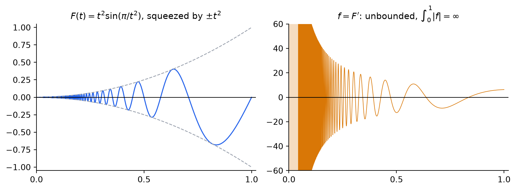
• \(f\) is not Lebesgue integrable. If it were, then, \(F\) being differentiable at every point with \(F'=f\in L^1[0,1]\), we would have \(F(x)=\int_0^x f\) for all \(x\) (Rudin 1987, chap. 7), so \(F\) would be absolutely continuous and in particular of bounded variation. But at \(t_k=(k+\tfrac{1}{2})^{-1/2}\) we have \(F(t_k)=\dfrac{(-1)^k}{k+\frac{1}{2}}\), so \(\sum_k|F(t_{k+1})-F(t_k)|\ge\sum_k\dfrac{1}{k+\frac{1}{2}}=\infty\).
• \(f\) is Kurzweil integrable, by Theorem 2, and \[ \int_0^1 f(t)\,dt=F(1)-F(0)=\sin\pi-0=0. \]

import matplotlib.pyplot as plt
import numpy as np


def F(t):
    return np.where(t > 0, t**2 * np.sin(np.pi / np.maximum(t, 1e-12) ** 2), 0.0)


def f(t):  # f = F'
    u = np.pi / np.maximum(t, 1e-12) ** 2
    return np.where(t > 0, 2 * t * np.sin(u) - 2 * np.pi / np.maximum(t, 1e-12) * np.cos(u), 0.0)


def phase_samples(t_min, t_max, per_osc=60):
    """Points equally spaced in the phase pi/t^2, so every oscillation gets the same number of points."""
    ph = np.linspace(np.pi / t_max**2, np.pi / t_min**2, int(per_osc * (1 / t_min**2 - 1 / t_max**2) / 2) + 200)
    return np.sort(np.sqrt(np.pi / ph))


BLUE, ORANGE, GREY = "#2563eb", "#d97706", "#9ca3af"
fig, (axF, axf) = plt.subplots(1, 2, figsize=(9, 3.4))

t = np.concatenate([[0.0], phase_samples(0.03, 1.0)])
axF.plot(t, F(t), color=BLUE, lw=1.2)
axF.plot(t, t**2, color=GREY, lw=1, ls="--")
axF.plot(t, -t**2, color=GREY, lw=1, ls="--")
axF.set_title(r"$F(t)=t^2\sin(\pi/t^2)$, squeezed by $\pm t^2$", fontsize=11)
axF.set_ylim(-1.05, 1.05)

t = phase_samples(0.045, 1.0)
axf.plot(t, f(t), color=ORANGE, lw=0.7)
axf.axvspan(0, 0.045, color=ORANGE, alpha=0.25, lw=0)
axf.set_ylim(-60, 60)
axf.set_title(r"$f=F'$: unbounded, $\int_0^1|f|=\infty$", fontsize=11)

for ax in (axF, axf):
    ax.axhline(0, color="black", lw=0.8)
    ax.set_xlim(0, 1.02)
    ax.set_xticks([0, 0.5, 1])
    ax.spines[["right", "top"]].set_visible(False)
fig.tight_layout()
plt.show()

Figure 4: Example 2. Left: \(F\) oscillates infinitely often near \(0\) but stays between \(\pm t^2\), so it is differentiable at \(0\). Right: its derivative \(f\) is unbounded (cut at \(\pm60\); the shaded strip near \(0\) hides infinitely many oscillations).

Watch it. Part I of the animation Kurzweil integral and generalized ODEs builds this section step by step: the statement of Theorem 2 and Example 2 start at 2:32, and the proof, where the derivative becomes the gauge, at 3:16.

Generalized ODEs

In what follows, let \(\mathcal{O}\subset X\) be an open set and \(I\subset\mathbb{R}\) a nonempty set. Setting \(\Omega=\mathcal{O}\times I\), we consider a map \(F\colon \Omega \to X\).

A function \(x\colon J\to X\), defined on an interval \(J\subset I\), is called a solution of the generalized ODE \[ \dfrac{dx}{d\tau} = DF(x,t) \tag{4}\] if \((x(t),t)\in \Omega\) for all \(t\in J\) and \[ x(t) - x(s) = \int_{s}^{t}DF(x(\tau),t), \quad \text{for all } t,s \in J. \] where the integral is in the sense of Definition 3, with \(U(\tau,t)=F(x(\tau),t)\).

Remark. The symbolic expression in (4) serves to define the generalized ODE implicitly through its solutions. In this context, the symbol ``\(D\)’’ signifies that integration is understood in the Kurzweil sense, setting \(U(\tau, t) = F(x(\tau), t)\). Consequently, the notation \(\frac{dx}{d\tau}\) does not imply differentiability of the solution.

To illustrate this, Schwabik considered a continuous, nowhere differentiable function \(r \colon \mathbb{R} \to \mathbb{R}\) and defined \(F \colon \mathbb{R}^2 \to \mathbb{R}\) by \(F(x,t) = r(t)\). Then, \(x(t) = r(t)\), \(t \in \mathbb{R}\), is a solution to the generalized ODE \[ \frac{dx}{d\tau} = D[r(t)] = DF(x,t), \] since \[ \int_{s_1}^{s_2} DF(x(\tau),t) = \int_{s_1}^{s_2} D r(t) = r(s_2) - r(s_1) \] for all \(s_1, s_2 \in \mathbb{R}\).

Next, we introduce a special class of functions \(F\colon\Omega\to X\), which allows us to establish, in particular, local existence and uniqueness of solutions to the generalized ODE (4), as will become clear in the sequel.

Definition 4 (The class \(\mathcal{F}(\Omega,h)\)) Let \(h\colon I\to \mathbb{R}\) be a nondecreasing function. A map \(F\colon\Omega\to X\) belongs to the class \(\mathcal{F}(\Omega,h)\) if, for all \(x,y\in \mathcal{O}\) and \(s_{1},s_{2}\in I\), \[\begin{align} \|F(x,s_{2})-F(x,s_{1})\| &\leq |h(s_{2})-h(s_{1})|, \\ \|F(x,s_{2})-F(x,s_{1})-F(y,s_{2})+F(y,s_{1})\| &\leq \|x-y\||h(s_{2})-h(s_{1})|. \end{align}\]

If \(F\in\mathcal{F}(\Omega,h)\), every solution of \(\frac{\mathrm{d}x}{\mathrm{d}\tau}=\mathrm{D}F(x,t)\) on \([a,b]\) satisfies \(\|x(s_2)-x(s_1)\|\le|h(s_2)-h(s_1)|\), so it is of bounded variation and it is continuous wherever \(h\) is (Bonotto et al. 2021, Lemma 4.9).

Theorem 3 (Existence and uniqueness) Assume that \(F\colon\Omega\to X\) belongs to the class \(\mathcal{F}(\Omega,h)\), where \(h\) is also left-continuous. If \((\widetilde{x},t_{0})\in\Omega\) is such that \[ \widetilde{x}{+} = \widetilde{x} +F(\widetilde{x},t_{0}^{+}) - F(\widetilde{x},t_{0})\in\mathcal{O}, \] then there exists a number \(\Delta>0\) such that, on the interval \([t_{0},t_{0}+\Delta]\), there exists a unique solution \(x\colon[t_{0},t_{0}+\Delta]\to \mathcal{O}\) of the generalized ODE (4) for which \(x(t_{0})=\widetilde{x}\).

The condition \(\widetilde{x} + F(\widetilde{x},t_{0}^{+}) - F(\widetilde{x},t_{0}) \in \mathcal{O}\) guarantees that after the jump (at the point of discontinuity), the corresponding solution remains in the open set \(\mathcal{O}\) and can be extended for \(t > t_{0}\). Furthermore, the assumption of left-continuity on \(h\) could be weakened by imposing the condition \[ x + F(x,t^{-}) - F(x,t) \in \mathcal{O}. \]

Measure differential equations as generalized ODEs

Throughout this section, \(O\subset X\) is open, \(t_0\in\mathbb{R}\), \(\sigma>0\), and \(\tau_0\geq t_0\). Consider an measure differential equation (MDE) whose integral form is given by \[ x(t) = x(\tau_0) + \int_{\tau_0}^{t}f(x(s),s)dg(s),\quad t\geq\tau_0, \tag{5}\] where \(f\colon O\times[t_{0},t_{0}+\sigma]\to X\) and \(g\colon[t_{0},t_{0}+\sigma]\to\mathbb{R}\) are functions, and the integral on the right-hand side is in the sense of Perron-Stieltjes.

In order to obtain the existence of solution for the MDE (5), we shall assume that \(f\colon O\times[t_{0},t_{0}+\sigma]\to X\) and \(g\colon[t_{0},t_{0}+\sigma]\to\mathbb{R}\) satisfies the following conditions (Bonotto et al. 2021, sec. 4.2):

(A1) \(g\) is nondecreasing and left-continuous.

(A2) The Perron–Stieltjes integral \(\int_{s_1}^{s_2} f(x(s),s)\,\mathrm{d}g(s)\) exists for all \(x\in G([t_0,t_0+\sigma],O)\) and all \(s_1,s_2\in[t_0,t_0+\sigma]\).

(A3) There is a function \(M\colon[t_0,t_0+\sigma]\to\mathbb{R}\), Perron–Stieltjes integrable with respect to \(g\), such that \[ \left\|\int_{s_1}^{s_2} f(x(s),s)\,\mathrm{d}g(s)\right\|\le\int_{s_1}^{s_2} M(s)\,\mathrm{d}g(s) \] for all \(x\in G([t_0,t_0+\sigma],O)\) and all \(t_0\le s_1\le s_2\le t_0+\sigma\).

(A4) There is a function \(L\colon[t_0,t_0+\sigma]\to\mathbb{R}\), Perron–Stieltjes integrable with respect to \(g\), such that \[ \left\|\int_{s_1}^{s_2} \left[f(x(s),s)-f(z(s),s)\right]\,\mathrm{d}g(s)\right\|\le\|x-z\|_\infty\int_{s_1}^{s_2} L(s)\,\mathrm{d}g(s) \] for all \(x,z\in G([t_0,t_0+\sigma],O)\) and all \(t_0\le s_1\le s_2\le t_0+\sigma\).

The idea now is to use conditions (A1)-(A4) above, to see a MDE as a generalized ODE and with this to obtain the existence and uniqueness of solution to a measure differential equation of the form (5).

Theorem 4 (MDEs are generalized ODEs) Assume functions \(f\) and \(g\) satisfies conditions (A1)–(A4). Fix \(\tau_0\in[t_0,t_0+\sigma]\), and define \(F\colon O\times[t_0,t_0+\sigma]\to X\) by \[ F(x,t)=\int_{\tau_0}^{t} f(x,s)\,\mathrm{d}g(s),\qquad (x,t)\in O\times[t_0,t_0+\sigma]. \tag{6}\]

Then, \(F\in\mathcal{F}(\Omega,h)\), where \(h\colon[t_0,t_0+\sigma]\to\mathbb{R}\) given by \[ h(t)=\int_{\tau_0}^{t}\left(M(s)+L(s)\right)\,\mathrm{d}g(s) \] is a nondecreasing function.

The next theorem is the key step: along a regulated function, the Kurzweil integral of \(F\) and the Perron–Stieltjes integral of \(f\) coincide (Bonotto et al. 2021, Theorem 4.13).

Theorem 5 (Kurzweil and Perron–Stieltjes integrals) Assume that \(f\colon O\times[t_0,t_0+\sigma]\to X\) satisfies conditions (A2)–(A4), that \(g\colon[t_0,t_0+\sigma]\to\mathbb{R}\) satisfies condition (A1), and let \(F\) be given by (6). If \(x\colon[t_0,t_0+\sigma]\to O\) is a regulated function (in particular, a function of bounded variation), then the Kurzweil integral \(\int_{t_0}^{t_0+\sigma}\mathrm{D}F(x(\tau),t)\) and the Perron–Stieltjes integral \(\int_{t_0}^{t_0+\sigma}f(x(s),s)\,\mathrm{d}g(s)\) both exist, and \[ \int_{t_0}^{t_0+\sigma}\mathrm{D}F(x(\tau),t)=\int_{t_0}^{t_0+\sigma}f(x(s),s)\,\mathrm{d}g(s). \tag{7}\]

As a consequence, measure differential equations and generalized ODEs have the same solutions (Bonotto et al. 2021, Theorem 4.14).

Theorem 6 (MDEs and generalized ODEs have the same solutions) Assume that \(f\) satisfies conditions (A2)–(A4), that \(g\) satisfies condition (A1), and let \(F\) be given by (6). Then \(x\colon I\to X\) is a solution of the MDE (5) on an interval \(I\subset[t_0,t_0+\sigma]\) if and only if \(x\) is a solution of the generalized ODE \[ \frac{\mathrm{d}x}{\mathrm{d}\tau}=\mathrm{D}F(x,t) \] on \(I\).

References

Bonotto, Everaldo M., Márcia Federson, and Jaqueline G. Mesquita, eds. 2021. Generalized Ordinary Differential Equations in Abstract Spaces and Applications. Wiley.

Gordon, Russell A. 1994. The Integrals of Lebesgue, Denjoy, Perron, and Henstock. Vol. 4. Graduate Studies in Mathematics. American Mathematical Society.

Henstock, Ralph. 1961. “Definitions of Riemann Type of the Variational Integrals.” Proceedings of the London Mathematical Society. Third Series 11: 402–18.

Kurzweil, Jaroslav. 1957. “Generalized Ordinary Differential Equations and Continuous Dependence on a Parameter.” Czechoslovak Mathematical Journal 7(82): 418–49.

Rudin, Walter. 1976. Principles of Mathematical Analysis. 3rd ed. McGraw-Hill.

Rudin, Walter. 1987. Real and Complex Analysis. 3rd ed. McGraw-Hill.

Schwabik, Štefan. 1992. Generalized Ordinary Differential Equations. Vol. 5. Series in Real Analysis. World Scientific.